How do I turn one EEG recording into a PyTorch DataLoader?

Estimated reading time:19 minutes

A model trains on tensor batches, not on continuous voltage traces. This tutorial closes the gap on one BIDS recording from OpenNeuro ds002718 [Wakeman and Henson, 2015], reachable through NEMAR [Delorme et al., 2022]: two safe preprocessors, a fixed-length window step, a DataLoader [Paszke et al., 2019], and an optional Zarr cache that turns batch reads into a few milliseconds of random access. We do not train a model. The deliverable is one batch’s shape and dtype.

Learning objectives

• Chain EEGDashDataset, braindecode.preprocessing.preprocess(), and create_fixed_length_windows() on one subject.

• Predict the shape of one window from (n_channels, window_seconds * sfreq) and verify it.

• Read one batch from torch.utils.data.DataLoader and explain each axis.

• Convert the windowed dataset to a Zarr store and re-read it for random-access speed.

• Pick safe values for batch_size, num_workers, pin_memory, and shuffle for an EEG workload.

Requirements

• About 2 min on CPU on first run; under 20 s once cached.

• Network on first call (~30-60 MB into cache_dir); offline thereafter.

• Prerequisites: How do I find datasets in EEGDash? (catalogue), How do I load one EEG recording from EEGDash? (one Raw).

• Concept: EEGDash objects: EEGDash, EEGDashDataset, EEGChallengeDataset.

Setup. np.random.seed and torch.manual_seed make shuffle=True and any model init reproducible across runs (E3.21).

import os
from pathlib import Path

import matplotlib.pyplot as plt
import numpy as np
import pandas as pd
import torch
from torch.utils.data import DataLoader

import braindecode
import eegdash
from braindecode.preprocessing import (
    Preprocessor,
    create_fixed_length_windows,
    preprocess,
)
from eegdash import EEGDashDataset
from eegdash.viz import use_eegdash_style

use_eegdash_style()
SEED = 42
np.random.seed(SEED)
torch.manual_seed(SEED)

CACHE_DIR = Path(os.environ.get("EEGDASH_CACHE_DIR", Path.home() / ".eegdash_cache"))
CACHE_DIR.mkdir(parents=True, exist_ok=True)
print(
    f"eegdash {eegdash.__version__}; braindecode {braindecode.__version__}; "
    f"torch {torch.__version__}"
)
print(f"cache_dir={CACHE_DIR}")

eegdash 0.7.2; braindecode 1.5.0; torch 2.11.0+cu130
cache_dir=/home/runner/eegdash_cache

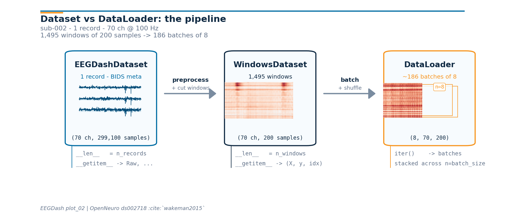
Dataset vs DataLoader: the mental model

PyTorch’s official tutorial draws the line clearly: a Dataset owns sample storage and retrieval (__len__ and __getitem__); a DataLoader consumes the dataset and adds batching, shuffling, and worker orchestration. The DataLoader is not a data store. It is an iterable that calls __getitem__ on the dataset behind it and stacks the results.

On EEG, the picture has three shapes you can keep in your head:

EEGDashDataset                  WindowsDataset                DataLoader
(records + BIDS meta)           (cut samples for the model)   (consumer)
┌────────────────────┐          ┌───────────────────┐         ┌────────────┐
│ record 0 (Raw) ──┐ │ preproc  │ window 0 (X, y)   │ batch + │ batch 0    │
│ record 1 (Raw) ──┼─┼─────────▶│ window 1 (X, y)   │ shuffle │ batch 1    │
│ record 2 (Raw) ──┘ │ + cut    │ ...               │────────▶│ ...        │
│ ...                │ windows  │ window N (X, y)   │         │ batch K    │
└────────────────────┘          └───────────────────┘         └────────────┘
  __len__  = n_records           __len__  = n_windows           iter() yields
  __getitem__ -> (raw, ...)       __getitem__ -> (X, y, idx)      stacked tensors

Once the pipeline runs, we re-draw this diagram further down with the live shapes that came out of the runtime.

Five corollaries

• A sample is a window, not a recording. Continuous EEG is one long array per session. Models train on fixed-length frames, so the pipeline cuts each Raw into (n_channels, window_samples) tensors before any batching happens.

• Pipeline composition. EEGDashDataset (records and BIDS metadata) feeds preprocess() (in-place edits on each mne.io.Raw) which feeds create_fixed_length_windows() (continuous, then windowed) which feeds DataLoader (windowed, then batched). Each stage carries the BIDS metadata forward, which keeps later splits subject-aware (see /auto_examples/tutorials/10_core_workflow/plot_11_leakage_safe_split).

• Two windowing surfaces. create_fixed_length_windows() strides across the continuous signal, ignoring events; useful for self-supervised pretraining and sleep staging. create_windows_from_events() cuts around BIDS event onsets with explicit offsets; this is the right choice for ERP and event-related tasks (face/scrambled, oddball, motor imagery). Both return a BaseConcatDataset of WindowsDataset and slot into the same DataLoader without any code change.

• Random access vs sequential storage. Training shuffles windows; the underlying signal store has to support cheap X[i] lookups. .fif is fine for one recording but its random-access cost grows linearly with file size; Zarr stores fixed-size chunks and reads any window in tens of milliseconds (see Step 5).

• Lazy by default. Building the dataset queries the metadata index. The MNE Raw is materialised on demand (record.raw). preload=True on the windowing helpers forces the cut signal into RAM, which is the right trade-off when the recording fits in memory.

• Connections back and forward. plot_01 opened the same record and inspected the spectrum. plot_10 covers the full preprocessing recipe (montage, reference, band-pass) we keep minimal here. plot_11 splits without leakage. plot_13 saves and reloads the prepared windows so subsequent sessions skip the cut.

What can a windowed dataset do?

Before building one, list the methods braindecode.datasets.WindowsDataset exposes; most of them are the verbs a DataLoader implicitly relies on (__len__, __getitem__, set_description, transform).

from braindecode.datasets import WindowsDataset

windows_methods = sorted(
    name
    for name in dir(WindowsDataset)
    if not name.startswith("_") and callable(getattr(WindowsDataset, name, None))
)
pd.DataFrame({"method": windows_methods}).head(20)

	method
0	set_description

Step 1: Build the dataset (lazy)

Same idiom as plot_01. One subject keeps the run inside the tutorial budget; the BIDS query language carries through unchanged [Pernet et al., 2019].

DATASET = "ds002718"
SUBJECT = "002"  # E3.23 data minimality: one subject, one task
TASK = "FaceRecognition"
dataset = EEGDashDataset(
    cache_dir=CACHE_DIR, dataset=DATASET, subject=SUBJECT, task=TASK
)
record = dataset.datasets[0]
raw = record.raw
pd.Series(
    {
        "n_recordings": len(dataset.datasets),
        "n_channels": raw.info["nchan"],
        "sfreq (Hz)": float(raw.info["sfreq"]),
        "duration (s)": round(raw.times[-1], 1),
    },
    name="value",
).to_frame()

Downloading sub-002_task-FaceRecognition_channels.tsv:   0%|          | 0.00/1.31k [00:00<?, ?B/s]
Downloading sub-002_task-FaceRecognition_channels.tsv: 100%|██████████| 1.31k/1.31k [00:00<00:00, 5.58MB/s]

Downloading sub-002_task-FaceRecognition_events.tsv:   0%|          | 0.00/105k [00:00<?, ?B/s]
Downloading sub-002_task-FaceRecognition_events.tsv: 100%|██████████| 105k/105k [00:00<00:00, 117MB/s]

Downloading sub-002_task-FaceRecognition_electrodes.tsv:   0%|          | 0.00/1.68k [00:00<?, ?B/s]
Downloading sub-002_task-FaceRecognition_electrodes.tsv: 100%|██████████| 1.68k/1.68k [00:00<00:00, 6.88MB/s]

Downloading sub-002_task-FaceRecognition_eeg.json:   0%|          | 0.00/1.28k [00:00<?, ?B/s]
Downloading sub-002_task-FaceRecognition_eeg.json: 100%|██████████| 1.28k/1.28k [00:00<00:00, 4.99MB/s]

Downloading sub-002_task-FaceRecognition_coordsystem.json:   0%|          | 0.00/283 [00:00<?, ?B/s]
Downloading sub-002_task-FaceRecognition_coordsystem.json: 100%|██████████| 283/283 [00:00<00:00, 1.09MB/s]
[05/08/26 18:41:34] WARNING  File not found on S3, skipping:   downloader.py:163
                             s3://openneuro.org/ds002718/sub-0
                             02/eeg/sub-002_task-FaceRecogniti
                             on_eeg.fdt

Downloading sub-002_task-FaceRecognition_eeg.set:   0%|          | 0.00/224M [00:00<?, ?B/s]
Downloading sub-002_task-FaceRecognition_eeg.set:  22%|██▏       | 50.0M/224M [00:01<00:05, 31.7MB/s]
Downloading sub-002_task-FaceRecognition_eeg.set: 100%|██████████| 224M/224M [00:01<00:00, 138MB/s]

	value
n_recordings	1.0
n_channels	74.0
sfreq (Hz)	250.0
duration (s)	2991.0

Step 2: Two safe preprocessors

Predict. What does raw.info['sfreq'] look like after a 100 Hz resample? And len(raw.ch_names) after dropping non-EEG channels?

Run. pick_types(eeg=True) keeps only EEG, resample(sfreq=100) downsamples. Filter and reference live in plot_10; here we keep the recipe to two named steps so the focus stays on the Raw -> windows -> DataLoader plumbing.

TARGET_SFREQ = 100  # Hz
preprocess(
    dataset,
    [
        Preprocessor("pick_types", eeg=True, eog=False, misc=False),
        Preprocessor("resample", sfreq=TARGET_SFREQ),
    ],
)
raw_pp = dataset.datasets[0].raw
n_channels = len(raw_pp.ch_names)
sfreq = float(raw_pp.info["sfreq"])
pd.Series(
    {
        "n_channels": n_channels,
        "sfreq (Hz)": sfreq,
        "dtype": str(raw_pp.get_data().dtype),
    },
    name="value",
).to_frame()

/home/runner/work/EEGDash/EEGDash/.venv/lib/python3.12/site-packages/braindecode/preprocessing/preprocess.py:78: UserWarning: apply_on_array can only be True if fn is a callable function. Automatically correcting to apply_on_array=False.
  warn(
NOTE: pick_types() is a legacy function. New code should use inst.pick(...).

	value
n_channels	70
sfreq (Hz)	100.0
dtype	float64

Step 3: Cut into fixed-length windows

Two parameters drive every shape from here on: window size and stride.

• window_size_samples = window_seconds * sfreq.

• window_stride_samples = window_size_samples gives 0 % overlap; each input sample lands in exactly one window.

• Halving the stride doubles the window count and introduces correlated frames inside one recording, which usually hurts evaluation unless the splits below stay subject-aware (cross-subject in plot_11).

Predict. len(windows) for a 1-second recording at 100 Hz with 2-second windows? (Answer: zero, after drop_last_window=True.)

WINDOW_SECONDS = 2.0
window_size_samples = int(WINDOW_SECONDS * TARGET_SFREQ)
windows = create_fixed_length_windows(
    dataset,
    window_size_samples=window_size_samples,
    window_stride_samples=window_size_samples,  # 0 % overlap
    drop_last_window=True,
    preload=True,
)
X_one, y_one, _idx = windows[0]
pd.Series(
    {
        "n_windows": len(windows),
        "windows[0][0].shape": str(tuple(X_one.shape)),
        "X.dtype": str(X_one.dtype),
        "window_samples": window_size_samples,
        "window_seconds": WINDOW_SECONDS,
    },
    name="value",
).to_frame()

	value
n_windows	1495
windows[0][0].shape	(70, 200)
X.dtype	float32
window_samples	200
window_seconds	2.0

Step 4: Wrap in a DataLoader

Four knobs matter on EEG; every other DataLoader argument can stay at default until the model trains.

• batch_size. 8-32 is a comfortable starting range for a CPU debug run; final-training values are dictated by GPU memory.

• shuffle. True for training, False for evaluation. True requires a seeded torch.Generator if the first batch must match across runs.

• num_workers. 0 (synchronous) is the right default with preload=True because windows already live in RAM. >0 helps only when the dataset reads from disk per __getitem__ (the Zarr path below).

• pin_memory. Set to True if a CUDA device is present and you plan to send batches with .to(device, non_blocking=True).

BATCH_SIZE = 8
gen = torch.Generator().manual_seed(SEED)
loader = DataLoader(
    windows,
    batch_size=BATCH_SIZE,
    shuffle=True,
    num_workers=0,
    pin_memory=torch.cuda.is_available(),
    generator=gen,
)
X_batch, y_batch, _idx_batch = next(iter(loader))
pd.Series(
    {
        "X.shape": str(tuple(X_batch.shape)),
        "X.dtype": str(X_batch.dtype),
        "y.shape": str(tuple(y_batch.shape)),
        "y unique": str(torch.unique(y_batch).tolist()),
        "pin_memory": loader.pin_memory,
        "num_workers": loader.num_workers,
    },
    name="value",
).to_frame()

	value
X.shape	(8, 70, 200)
X.dtype	torch.float32
y.shape	(8,)
y unique	[-1]
pin_memory	False
num_workers	0

Investigate. The batch tensor is shaped (batch_size, n_channels, window_size_samples) with floating-point dtype. That is exactly what Braindecode models such as ShallowFBCSPNet and EEGNetv4 consume.

Pipeline at a glance: the live shapes

Now that every stage has run, we can re-draw the mental-model diagram from the top with the actual numbers the runtime produced. The drawing helpers live in a sibling _pipeline_diagram module so the rendering plumbing stays out of this tutorial; the call below is the only line that matters.

from _pipeline_diagram import draw_pipeline

fig_pipe = draw_pipeline(
    record_signal=raw_pp.get_data(picks="eeg").copy(),
    window_xy=np.asarray(windows[0][0]).copy(),
    batch_xy=np.asarray(X_batch[0]).copy(),
    n_records=len(windows.datasets),
    n_channels=n_channels,
    sfreq=sfreq,
    window_size_samples=window_size_samples,
    batch_size=BATCH_SIZE,
    n_windows=len(windows),
    subject=SUBJECT,
    n_channels_full=raw_pp.info["nchan"],
)
plt.show()

Reproducibility: which random source draws which window?

Two seeds and one Generator cover the failure modes that bite EEG pipelines.

• np.random.seed and torch.manual_seed make the main process deterministic: model init, baseline shuffle=True ordering when num_workers=0, and any NumPy use inside the dataset’s __getitem__.

• A torch.Generator passed to the DataLoader fixes the sampling order. Without it, two shuffle=True runs see different windows in the first batch. torch.manual_seed alone is not enough because PyTorch advances the global generator from any other operation that touches it.

• With num_workers > 0, each worker forks the parent state. NumPy does not re-seed automatically (PyTorch does, with a deterministic per-worker seed). The canonical fix is the seed_worker(worker_id) template below; this is what PyTorch’s own reproducibility guide recommends.

import random


def seed_worker(worker_id):
    """Re-seed numpy and stdlib random in each DataLoader worker."""
    worker_seed = torch.initial_seed() % 2**32
    np.random.seed(worker_seed)
    random.seed(worker_seed)


loader_repro = DataLoader(
    windows,
    batch_size=BATCH_SIZE,
    shuffle=True,
    num_workers=0,  # set >0 once the dataset reads from disk per __getitem__
    pin_memory=torch.cuda.is_available(),
    worker_init_fn=seed_worker,
    generator=torch.Generator().manual_seed(SEED),
)


def _first_batch_indices(loader):
    """Return the per-window i_start indices of the first batch as a list."""
    _, _, idx_batch = next(iter(loader))
    arr = np.asarray(idx_batch)
    if arr.ndim >= 2:
        return arr[:, 1].tolist()  # i_start_in_trial column
    return list(arr)


first_idx_a = _first_batch_indices(loader_repro)
first_idx_b = _first_batch_indices(
    DataLoader(
        windows,
        batch_size=BATCH_SIZE,
        shuffle=True,
        num_workers=0,
        worker_init_fn=seed_worker,
        generator=torch.Generator().manual_seed(SEED),
    )
)
pd.Series(
    {
        "first batch indices (run A)": str(first_idx_a),
        "first batch indices (run B)": str(first_idx_b),
        "match?": first_idx_a == first_idx_b,
    },
    name="value",
).to_frame()

	value
first batch indices (run A)	[455, 91000, 91200]
first batch indices (run B)	[455, 91000, 91200]
match?	True

Step 5: Unlock random-access speed with Zarr

preload=True keeps windows in RAM, which is the right answer for a tutorial. For real training the dataset rarely fits in memory, and .fif files become the bottleneck (sequential format, one recording per file, no chunked random access). Braindecode’s solution is a Zarr store: fixed-size chunks, Blosc compression, and an __getitem__ that reads one window in tens of milliseconds even when the full dataset is hundreds of GB.

The conversion is the same code path that push_to_hub() runs locally before the Hub upload; we use it offline here. Run this section once per project: subsequent loads pay the chunk-decode cost only, not the recompute cost. The reload returns the same BaseConcatDataset API so the DataLoader code above is unchanged.

Note

Zarr is an optional Braindecode extra. Install it once into the same environment:

pip install braindecode[hub]

# Convert windows to a Zarr-backed cache (one-time, ~seconds for
# one recording, scales linearly with dataset size):
from braindecode.datasets import BaseConcatDataset

zarr_dir = CACHE_DIR / "ds002718_windows.zarr"
windows.push_to_hub(
    repo_id="local-only/ds002718-windows",
    local_cache_dir=zarr_dir,
    compression="blosc",   # blosc > zstd > gzip for random reads
    compression_level=5,    # 5 is the documented sweet spot
    chunk_size=5_000_000,   # samples per chunk; one chunk = one read
    token=None,
)

# Reload as a BaseConcatDataset; the DataLoader API is unchanged.
windows_zarr = BaseConcatDataset.pull_from_hub(
    repo_id="local-only/ds002718-windows",
    cache_dir=zarr_dir,
    preload=False,            # lazy reads from chunks
)

Trade-offs. Blosc beats Zstd and Gzip on random-read latency at the cost of larger files. chunk_size tunes the read amplification: a small chunk reads quickly but pays per-chunk metadata overhead; a large chunk amortises that cost but reads more bytes than the model asked for. The default of 5 M samples is conservative for one-second windows at 100 Hz. With Zarr in place, DataLoader(num_workers=4, pin_memory=True) becomes the right default rather than an over-eager guess.

A common mistake, and how to recover

Run. Asking for windows larger than the recording silently returns zero. We trigger it on purpose so the failure mode is visible [Nederbragt et al., 2020]: a DataLoader(empty) quietly yields nothing, which masks the bug.

huge = int(raw_pp.times[-1] * TARGET_SFREQ * 10)  # 10x recording length
try:
    bad = create_fixed_length_windows(
        dataset,
        window_size_samples=huge,
        window_stride_samples=huge,
        drop_last_window=True,
        preload=True,
    )
    print(f"Oversize window produced len={len(bad)} (expected 0).")
except (ValueError, RuntimeError) as exc:
    print(f"Caught {type(exc).__name__}: {str(exc)[:120]}")
print(f"Recovery: keep window_size_samples={window_size_samples} (<< recording).")

Caught ValueError: Window size 2990990 exceeds trial duration 299100.
Recovery: keep window_size_samples=200 (<< recording).

Modify

Your turn. Set WINDOW_SECONDS = 4.0 and rerun Step 3 + Step 4. Predict before running: how should windows[0][0].shape[1] change? How should len(windows) change?

Make

Mini-project. Write a custom collate_fn that returns a dict instead of the default tuple. Dict batches stay readable when the pipeline grows beyond (X, y, idx): HuggingFace Trainer, Lightning LightningDataModule, and any code that calls model(**batch) expects keyword inputs, and dict keys document the tensor’s role at the call site rather than relying on positional convention.

def dict_collate(batch):
    """Stack a list of ``(X, y, idx)`` items into a keyed batch dict."""
    return {
        "signal": torch.stack(
            [torch.as_tensor(item[0], dtype=torch.float32) for item in batch], dim=0
        ),
        "target": torch.as_tensor([item[1] for item in batch]),
        "index": torch.as_tensor(
            [
                int(item[2][0])
                if isinstance(item[2], (list, tuple, np.ndarray))
                else int(item[2])
                for item in batch
            ]
        ),
    }


loader_dict = DataLoader(
    windows,
    batch_size=BATCH_SIZE,
    shuffle=False,
    num_workers=0,
    collate_fn=dict_collate,
)
batch = next(iter(loader_dict))
pd.Series(
    {
        "type(batch)": type(batch).__name__,
        "keys": str(sorted(batch.keys())),
        "signal.shape": str(tuple(batch["signal"].shape)),
        "signal.dtype": str(batch["signal"].dtype),
        "target.shape": str(tuple(batch["target"].shape)),
        "index.shape": str(tuple(batch["index"].shape)),
    },
    name="value",
).to_frame()

	value
type(batch)	dict
keys	['index', 'signal', 'target']
signal.shape	(8, 70, 200)
signal.dtype	torch.float32
target.shape	(8,)
index.shape	(8,)

Investigate. model(**batch) now passes signal=..., target=..., index=... as keyword arguments. That matches the convention used by HuggingFace Trainer and PyTorch Lightning data modules without any glue code.

Continuous windows vs event-based epochs

Underneath every WindowsDataset sits an mne.Epochs (or mne.EpochsArray) object: a 3-D array shaped (n_epochs, n_channels, n_times) plus an event_id dict that maps condition strings to integer codes ({'face': 1, 'scrambled': 2}) and an optional metadata pandas.DataFrame that lets you write trial-level filters such as epochs[epochs.metadata.task == 'face']. Raw is one continuous array; Epochs is already cut, with its own event_id / metadata / drop_bad machinery [Gramfort et al., 2013].

Two functions take you from Raw to that shape; the DataLoader does not care which one ran.

• create_fixed_length_windows() strides over the continuous signal and labels every window with the same description-derived target. Right call for self-supervised pretraining (no event labels needed), sleep staging (one stage per 30 s window), and monitoring tasks where the recording is labelled at the session level.

• create_windows_from_events() reads mne.io.Raw.annotations (BIDS events.tsv is loaded automatically by EEGDash), pulls a window of fixed length around each event onset using trial_start_offset_samples / trial_stop_offset_samples, and uses the event code as the target. Right call for ERP and event-related decoding (face vs scrambled in ds002718, P300 oddball, motor imagery cues). Pass mapping={'face': 0, 'scrambled': 1} to relabel at construction time without touching the underlying epochs object.

The DataLoader code from Step 4 is byte-identical in both cases. Switching is one line in the windowing call.

Changing the label without rebuilding the windows

The most-missed edit: the target in WindowsDataset is a column called "target" on a per-record pandas.DataFrame (the mne.Epochs metadata). __getitem__ reads self.y[index], which was populated from that column at construction. Three patterns cover the practical cases.

Pattern 0: use a BIDS field as the target. EEGDash pushes BIDS entities (subject, task, session, run, age, gender, sex, plus any participants.tsv extras) onto each record’s description at dataset construction. The braindecode windowing step then folds those values into braindecode.datasets.BaseConcatDataset.get_metadata() (one row per window), so picking a column out of that DataFrame is the whole adapter — y = metadata[col].to_numpy() is what feeds MOABB stratified splitters.

Pattern 1: relabel in place. Mutate the metadata column and the parallel y list on every per-record subdataset. Lasts for the Python session; no preprocessing rerun. Right call when the target is computed from the windows themselves (a sliding-window stage label the BIDS sidecar does not carry).

Pattern 2: map at construction time (event-based windows). Pass mapping={'face': 0, 'scrambled': 1} to create_windows_from_events(). The integer codes land in metadata['target'] directly.

Pattern 0: read BIDS fields as a target without any mutation. windows.get_metadata() is the braindecode adapter: one row per window, with the per-record description columns merged in. Picking a column gives the per-window target.

metadata = windows.get_metadata()
y_subject = metadata["subject"].to_numpy()
pd.Series(
    {
        "rows in metadata": len(metadata),
        "task unique": str(metadata["task"].unique().tolist()),
        "subject unique": str(metadata["subject"].unique().tolist()),
        "y_subject dtype": str(y_subject.dtype),
        "windows.datasets[0].description['task']": str(
            windows.datasets[0].description.get("task")
        ),
    },
    name="value",
).to_frame()

	value
rows in metadata	1495
task unique	['FaceRecognition']
subject unique	['002']
y_subject dtype	object
windows.datasets[0].description['task']	FaceRecognition

Investigate. Every window inherited the recording’s task / subject from the BIDS-merged description without touching windows.datasets[i].metadata['target']. The same call with target="age" would expose the participants.tsv age column; with target="group" (when present) it would expose the clinical group label. This is what /auto_examples/tutorials/10_core_workflow/plot_11_leakage_safe_split leans on for subject-aware MOABB splits.

Pattern 1: relabel in place

Right call when the label cannot come from a BIDS field on the description: a self-supervised pretext label, a sliding-window stage tag, or a teacher-model output.

Pattern 1: relabel one recording in place. First half gets label 0, second half label 1. The DataLoader picks up the new targets without any rebuild, and windows.get_metadata()['target'] would now return these mutated values.

sub_ds = windows.datasets[0]
n = len(sub_ds)
half = n // 2
new_targets = [0] * half + [1] * (n - half)
sub_ds.y = new_targets
sub_ds.metadata.loc[:, "target"] = new_targets

loader_relabelled = DataLoader(
    windows, batch_size=BATCH_SIZE, shuffle=False, num_workers=0
)
_, y_relabelled, _ = next(iter(loader_relabelled))
pd.Series(
    {
        "before (orig)": "all windows shared the recording-level target",
        "after y": str(torch.unique(y_relabelled).tolist()),
        "first 8 windows": str(new_targets[:8]),
    },
    name="value",
).to_frame()

	value
before (orig)	all windows shared the recording-level target
after y	[0]
first 8 windows	[0, 0, 0, 0, 0, 0, 0, 0]

Investigate. y.unique() flipped from a single value to [0, 1]. The metadata mutation is what carried the change forward; the in-RAM Raw array is untouched and the cache file on disk is untouched.

A common pitfall. Mutating y without updating metadata['target'] works for read-only iteration but breaks any downstream code (leakage-aware splits, Hub upload) that consults the metadata frame instead of the list. Change both together.

Result

We turned one subject of ds002718 into a reproducible PyTorch DataLoader: BIDS query, two safe preprocessors, fixed-length windowing, batched read. The first batch is shaped (batch_size, n_channels, window_samples) with floating-point dtype. A clean batch shape only confirms plumbing; signal quality and task design are still open questions [Cisotto and Chicco, 2024].

Wrap-up

We went from a single-record EEGDashDataset to a DataLoader, named the four knobs that matter, and pointed at the Zarr path that unlocks random-access speed once the project outgrows one recording in RAM. Next: /auto_examples/tutorials/10_core_workflow/plot_10_preprocess_and_window replaces the two safe preprocessors with the full montage / reference / filter / resample recipe; /auto_examples/tutorials/10_core_workflow/plot_11_leakage_safe_split splits the windows without leakage; /auto_examples/tutorials/10_core_workflow/plot_13_save_and_reuse_prepared_data saves and reloads the windows so subsequent sessions skip the cut.

Try it yourself

• Re-run with shuffle=True and generator=None: the first batch becomes non-deterministic across runs. Add the seeded torch.Generator back and re-verify.

• Set num_workers=2 and confirm the batch shape is identical while wall-time changes; explain why on a 1-2-core CPU.

• Replace window_stride_samples = window_size_samples with a 50 % overlap (window_size_samples // 2) and predict the new len(windows). Then verify your prediction.

• Run the Zarr conversion code block on a local path (repo_id="local-only/<name>"); compare random-read latency against the in-RAM DataLoader.

References

See References for the centralised bibliography of papers cited above. Add or amend an entry once in docs/source/refs.bib; every tutorial inherits the update.