How do I find datasets in EEGDash?

Estimated reading time:9 minutes

EEGDash exposes a metadata index over hundreds of BIDS-curated EEG datasets, served by the public REST API at https://data.eegdash.org. The same catalogue powers NEMAR, the EEGLAB-ecosystem portal that hosts EEG/MEG datasets with browsing, compute, and provenance tools (Delorme et al., 2022). The EEGDash client searches, filters, and summarises that index without downloading a single sample.

Learning objectives

• Open an EEGDash client and discover its public methods.

• Search records with multiple filter fields (BIDS entities + scientific metadata).

• Convert query results into a pandas.DataFrame for analysis.

• Compute cohort statistics (subjects, sampling rates, modalities) from metadata only.

Requirements

• About 1 minute on CPU; metadata only (< 5 MB on the wire).

• Network required; EEGDash consumes the public API at https://data.eegdash.org. No authentication is needed for read access.

Setup. No randomness here, so no seed.

import matplotlib.pyplot as plt
import pandas as pd

import eegdash
from eegdash import EEGDash
from eegdash.viz import EEGDASH_BLUE, style_figure, use_eegdash_style

use_eegdash_style()
print(f"eegdash {eegdash.__version__}")

eegdash 0.7.2

Step 1: Discover the EEGDash client

EEGDash() wraps the REST endpoint. dir() is faster than the docs.

Predict. A read-only catalogue client should expose at least three verbs: count, find, get. How many does EEGDash actually have?

Run. Print the public method list.

client = EEGDash()
public_methods = sorted(
    m for m in dir(client) if not m.startswith("_") and callable(getattr(client, m))
)
print(f"EEGDash() exposes {len(public_methods)} public methods:")
for m in public_methods:
    print(f"  - {m}")

EEGDash() exposes 10 public methods:
  - count
  - exists
  - find
  - find_datasets
  - find_one
  - get_dataset
  - insert
  - search_datasets
  - update_dataset
  - update_field

Investigate. count, exists, find, find_one, find_datasets, search_datasets, get_dataset, plus three admin verbs. find and find_datasets are the read paths we use throughout the gallery.

Step 2: How big is the catalogue?

count runs server-side and is the cheapest call we can make.

n_records = client.count({})
print(f"records in the index: {n_records:,}")

records in the index: 305,393

Step 3: A broad scan vs. a targeted query

Unfiltered find({}) returns a lightweight projection: BIDS entities only, no signal-shape fields. A dataset filter unlocks the full record (sampling rate, channel count, duration in samples).

Run both and compare the columns.

broad = pd.DataFrame(client.find({}, limit=200)).drop(columns=["_id"], errors="ignore")
focused = pd.DataFrame(
    client.find(
        {"dataset": {"$in": ["ds002718", "ds005514", "ds005863", "ds003061"]}},
        limit=200,
    )
).drop(columns=["_id"], errors="ignore")
print(f"broad   : {broad.shape[0]} rows x {broad.shape[1]} cols")
print(f"focused : {focused.shape[0]} rows x {focused.shape[1]} cols")
extra = sorted(set(focused.columns) - set(broad.columns))
print(f"extra columns when filtered: {extra}")

broad   : 200 rows x 16 cols
focused : 200 rows x 22 cols
extra columns when filtered: ['_has_missing_files', 'ch_names', 'montage_hash', 'nchans', 'ntimes', 'participant_tsv', 'sampling_frequency']

Step 4: What does one record actually contain?

A record is a metadata document, one row per BIDS file, not the samples themselves. The fields cover BIDS entities (subject, task, session, run), scientific metadata (sampling rate, channel count, duration in samples) and storage hints (relative path, datatype). Per the EEG-BIDS spec (Pernet et al. 2019, doi:10.1038/s41597-019-0104-8), every recording exposes these fields.

fields = [
    "dataset",
    "subject",
    "task",
    "session",
    "run",
    "sampling_frequency",
    "nchans",
    "ntimes",
    "datatype",
]
sample = focused.iloc[0]
record_view = sample[fields].to_frame("value")
record_view.loc["duration (s)"] = round(
    sample["ntimes"] / sample["sampling_frequency"], 1
)
record_view

	value
dataset	ds002718
subject	019
task	FaceRecognition
session	None
run	NaN
sampling_frequency	250.0
nchans	74
ntimes	743250
datatype	eeg
duration (s)	2973.0

Step 5: Cohort analysis on the DataFrame

value_counts, groupby, and describe cover most catalogue questions; the EEGDash client stays out of the way.

Records per dataset.

focused["dataset"].value_counts().to_frame("records")

	records
dataset
ds005514	143
ds003061	39
ds002718	18

Sampling-rate distribution.

focused["sampling_frequency"].value_counts().head(8).to_frame("records")

	records
sampling_frequency
500.0	143
256.0	39
250.0	18

Top tasks.

focused["task"].value_counts().head(8).to_frame("records")

	records
task
P300	39
contrastChangeDetection	31
surroundSupp	20
FaceRecognition	18
RestingState	14
FunwithFractals	13
DespicableMe	13
DiaryOfAWimpyKid	13

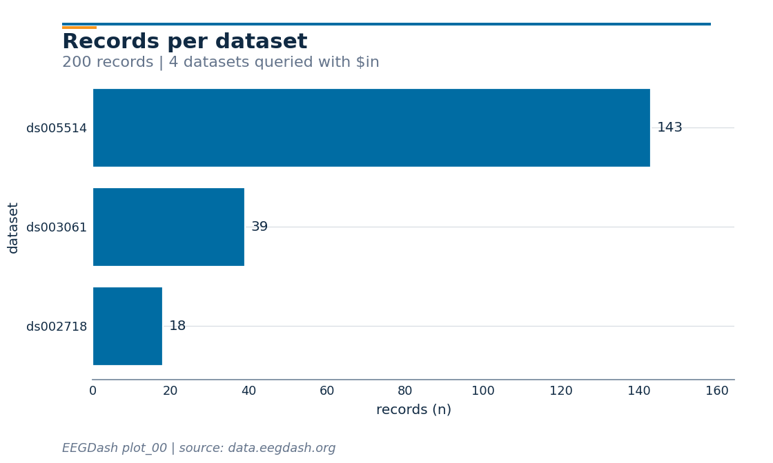
Step 6: Visualise the cohort

A horizontal bar of “records per dataset” reads at a glance.

counts = focused["dataset"].value_counts().iloc[::-1]
fig, ax = plt.subplots(figsize=(7, 4.2))
bars = ax.barh(counts.index, counts.values, color=EEGDASH_BLUE)
ax.bar_label(bars, padding=4, fontsize=9, color="#102A43")
ax.set_xlabel("records (n)")
ax.set_ylabel("dataset")
ax.set_xlim(0, counts.max() * 1.15)
style_figure(
    fig,
    title="Records per dataset",
    subtitle=f"{len(focused)} records | 4 datasets queried with $in",
    source="EEGDash plot_00 | source: data.eegdash.org",
)
plt.show()

Step 7: Dataset-level documents

find_datasets returns the catalogue documents (one per dataset) with DOI, BIDS version, demographics, and citation counts. Promote them to a DataFrame and shortlist by subject count.

catalogue = pd.DataFrame(client.find_datasets({}, limit=300))
catalogue["n_subjects"] = catalogue["demographics"].apply(
    lambda d: (d or {}).get("subjects_count", 0) if isinstance(d, dict) else 0
)
shortlist = (
    catalogue.loc[catalogue["n_subjects"] >= 5, ["dataset_id", "n_subjects", "license"]]
    .sort_values("n_subjects", ascending=False)
    .head(10)
    .reset_index(drop=True)
)
shortlist

	dataset_id	n_subjects	license
0	ds004395	364	CC0
1	ds004789	273	CC0
2	ds004809	252	CC0
3	ds002181	226	CC0
4	ds004602	182	CC0
5	ds004883	172	CC0
6	ds003655	156	CC0
7	ds004118	156	CC0
8	ds004584	149	CC0
9	ds004580	147	CC0

A common mistake, and how to recover

Run. Passing an unknown task name returns an empty list, not an error. The recovery is to surface what tasks the catalogue actually carries [Nederbragt et al., 2020].

unknown = client.find(task="FacePerceptionXYZ", limit=5)
print(f"records for unknown task: {len(unknown)}")
known_tasks = sorted(focused["task"].dropna().unique())[:8]
print(f"known tasks (first 8): {known_tasks}")

records for unknown task: 0
known tasks (first 8): ['DespicableMe', 'DiaryOfAWimpyKid', 'FaceRecognition', 'FunwithFractals', 'P300', 'RestingState', 'ThePresent', 'contrastChangeDetection']

Modify

Your turn. Combine filters: try client.find(task="RestingState", sampling_frequency=250, limit=20), then add subject="012". The query language is keyword-style for simple cases and Mongo-style ({"$gte": 250}) for ranges.

combined = client.find(task="RestingState", limit=20)
print(f"records for task=RestingState: {len(combined)}")

records for task=RestingState: 20

Make

Mini-project. Build a candidate cohort: pick a sampling-rate range and a minimum subject count, then return a DataFrame with [dataset_id, n_subjects, sampling_rates_seen]. Starter below.

def candidate_cohort(min_subjects: int = 5, sfreq_min: float = 200.0) -> pd.DataFrame:
    """Shortlist EEG datasets with >= ``min_subjects`` and at least one sampling rate >= ``sfreq_min``."""
    rates_per_dataset = (
        focused.groupby("dataset")["sampling_frequency"].agg(set).rename("rates")
    )
    out = catalogue.merge(
        rates_per_dataset,
        left_on="dataset_id",
        right_index=True,
        how="left",
    )
    out["max_sfreq"] = out["rates"].apply(
        lambda s: max(s) if isinstance(s, set) and s else 0.0
    )
    return (
        out.loc[
            (out["n_subjects"] >= min_subjects) & (out["max_sfreq"] >= sfreq_min),
            ["dataset_id", "n_subjects", "max_sfreq"],
        ]
        .sort_values(["n_subjects", "max_sfreq"], ascending=[False, False])
        .head(10)
    )


candidate_cohort(min_subjects=5, sfreq_min=200.0)

	dataset_id	n_subjects	max_sfreq
23	ds002718	18	250.0
41	ds003061	13	256.0

Result

We surveyed the EEGDash index without pulling a single sample, ran multi-field queries, and shortlisted candidate datasets in a DataFrame.

Wrap-up

Next: plot_01_first_recording.py actually downloads one record from the shortlist above and inspects its raw signal, channels, and duration.

Try it yourself

• Swap client.count({}) for client.count({"datatype": "eeg"}).

• Group df by dataset and report ntimes.sum() / sampling_frequency to get total recorded hours per dataset.

• Persist your shortlist with shortlist.to_parquet("candidates.parquet").

References

See References for the centralised bibliography of papers cited above. Add or amend an entry once in docs/source/refs.bib; every tutorial inherits the update.