How do I adapt a pretrained EEG model to a new task?

Estimated reading time:8 minutes

A pretrained EEG encoder packs hundreds of hours of recordings into a weight matrix. Paying the pretraining cost a second time is wasteful, training from scratch wastes the encoder. The decision in between is the fine-tuning regime: which slice of the network learns on the new task, and which slice stays pinned. This tutorial wires three regimes against a leakage-safe cross-subject split and reports per-epoch validation curves, final accuracy, and trainable parameter cost on one figure. The data come through a synthetic pretrain/target pair sized to mirror an OpenNeuro recording cataloged on NEMAR (Delorme et al. 2022, doi:10.1038/s41597-022-01795-4); the recipe transfers to any EEGDash windowed dataset by swapping synth_windows for an EEGDashDataset query. The three regimes: from-scratch (no pretrain weights, whole network trains), linear-probe (pretrained encoder frozen; only the head receives gradients; Banville et al. 2021, doi:10.1088/1741-2552/abca18), and full-finetune (encoder loaded, head reset, every parameter trains; Defossez et al. 2023, doi:10.1038/s42256-023-00714-5). The deliverable is a 3-panel figure plus a JSON line recording which regime won. So which one wins?

Learning objectives

• Train a small Braindecode encoder on a synthetic source task and save its weights.

• Build a leakage-safe cross-subject split with assert_no_leakage.

• Configure three fine-tuning regimes and verify frozen + trainable == total.

• Compare regimes with torch.optim.AdamW across seeds and read the 3-panel figure.

Requirements

• Estimated time: ~60 s on CPU, ~15 s on GPU.

• Data downloaded: 0 MB (synthetic windows; deterministic seed).

• Prerequisites: Pretrain on resting-state, fine-tune on contrast-change detection (encoder snapshot), /auto_examples/tutorials/10_core_workflow/plot_11_leakage_safe_split (cross-subject split).

• Concept page: Features vs. deep learning.

Seeding numpy and torch makes the printed accuracy and the rendered curves byte-stable across reruns (E3.21).

import json
import os
from pathlib import Path

import matplotlib.pyplot as plt
import numpy as np
import pandas as pd

from collections import Counter
from eegdash.viz import use_eegdash_style

use_eegdash_style()
SEED = 42
np.random.seed(SEED)

cache_dir = Path(os.environ.get("EEGDASH_CACHE_DIR", Path.cwd() / "eegdash_cache"))
cache_dir.mkdir(parents=True, exist_ok=True)
ckpt_path = cache_dir / "plot_73_pretrained_encoder.pt"

import torch
import torch.nn as nn
from braindecode.models import ShallowFBCSPNet

torch.manual_seed(SEED)

<torch._C.Generator object at 0x7f363891c8d0>

Three regimes, one figure: the mental model

The regimes differ only in which parameters carry a gradient on the target task. Architecture, data, optimiser, and seeds are held constant:

pretrained encoder weights      target task (small, leakage-safe)
+-------+---------------+        +----------------------------+
| encoder block | head |  --->   | from-scratch  : all train  |
+-------+---------------+        | linear-probe  : head only  |
                                 | full-finetune : all train  |
                                 +----------------------------+

from-scratch vs full-finetune (same parameter count, different starting weights) measures whether pretraining helped. linear-probe vs full-finetune (same starting weights, different trainables) measures how much the pretrained features want to move. Chance sits on every panel: reporting accuracy without it hides half the answer (Cisotto & Chicco 2024, doi:10.7717/peerj-cs.2256, Tip 9).

What does ShallowFBCSPNet expose?

List the named parameters so the freeze step has something to point at. The encoder is everything except final_layer; the linear-probe regime walks this list and toggles requires_grad.

_peek = ShallowFBCSPNet(8, 2, n_times=256, final_conv_length="auto")
print(
    pd.DataFrame(
        [
            {"name": n, "shape": tuple(p.shape), "n_params": p.numel()}
            for n, p in _peek.named_parameters()
        ]
    ).to_string(index=False)
)
del _peek

                              name          shape  n_params
   conv_time_spat.conv_time.weight (40, 1, 25, 1)      1000
     conv_time_spat.conv_time.bias          (40,)        40
   conv_time_spat.conv_spat.weight (40, 40, 1, 8)     12800
                      bnorm.weight          (40,)        40
                        bnorm.bias          (40,)        40
final_layer.conv_classifier.weight (2, 40, 11, 1)       880
  final_layer.conv_classifier.bias           (2,)         2

Step 1: Pretrain a small encoder on a synthetic source task

A real foundation model is pretrained on thousands of hours of recordings (Banville et al. 2021, doi:10.1088/1741-2552/abca18; Defossez et al. 2023, doi:10.1038/s42256-023-00714-5). Standing in here: a 6-subject synthetic task, two epochs of ShallowFBCSPNet, weights saved so Step 3 reloads them like from_pretrained. 8 channels and 2 s windows @ 128 Hz keep source/target shapes identical, which any transfer recipe demands (Schirrmeister et al. 2017, doi:10.1002/hbm.23730).

N_CHANS, N_TIMES, SFREQ = 8, 256, 128.0
PRETRAIN_TASK = "alpha-vs-delta-source"
TARGET_TASK = "alpha-vs-delta-target"

def synth_windows(n_subj, n_per, prefix="src", freq_offset=0.0, snr=2.0):
    """Two-class alpha-vs-delta windows with tunable signal-to-noise.

    Labels encode the dominant rhythm (10 Hz vs 2 Hz). ``freq_offset``
    nudges the carriers so the source encoder is helpful but not
    perfect; ``snr`` widens or closes the regime gap (Banville et al.
    2021, doi:10.1088/1741-2552/abca18).
    """
    rng = np.random.default_rng(SEED)
    t = np.arange(N_TIMES) / SFREQ
    X_list, rows = [], []
    for s in range(n_subj):
        labels = rng.integers(0, 2, size=n_per)
        # Per-subject amplitude jitter mimics electrode impedance.
        amp = snr * (0.6 + 0.08 * s)
        for w, lab in enumerate(labels):
            base = rng.standard_normal((N_CHANS, N_TIMES)).astype(np.float32)
            freq = (10.0 if lab == 1 else 2.0) + freq_offset
            base += amp * np.sin(2 * np.pi * freq * t).astype(np.float32)
            X_list.append(base)
            rows.append(
                {
                    "sample_id": f"{prefix}_s{s:02d}_w{w:03d}",
                    "subject": f"sub-{s:02d}",
                    "label": int(lab),
                }
            )
    return np.stack(X_list), np.array([r["label"] for r in rows]), pd.DataFrame(rows)


def build_model(n_outputs=2):
    return ShallowFBCSPNet(
        n_chans=N_CHANS, n_outputs=n_outputs, n_times=N_TIMES, final_conv_length="auto"
    )


# A high-SNR source gives the encoder useful inductive bias; the target
# lowers the SNR so the regime gap is visible.
X_src, y_src, _ = synth_windows(n_subj=6, n_per=40, prefix="src", snr=2.0)
print(f"source X={X_src.shape}, y={y_src.shape}")

source X=(240, 8, 256), y=(240,)

def evaluate(model, X, y):
    """Classification accuracy on ``(X, y)``."""
    model.eval()
    with torch.no_grad():
        preds = model(torch.from_numpy(X).float()).argmax(dim=1).numpy()
    return float((preds == y).mean())


def adamw_loop(model, X_tr, y_tr, *, epochs, lr, batch=32, X_val=None, y_val=None):
    """:class:`torch.optim.AdamW` loop with optional per-epoch validation.

    With ``X_val`` the return is per-epoch validation accuracy; without,
    per-epoch training loss. The figure consumes the validation form.
    """
    params = [p for p in model.parameters() if p.requires_grad]
    opt = torch.optim.AdamW(params, lr=lr, weight_decay=1e-4)
    loss_fn = nn.CrossEntropyLoss()
    Xt = torch.from_numpy(X_tr).float()
    yt = torch.from_numpy(y_tr).long()
    track = []
    for _ in range(epochs):
        model.train()
        idx = torch.randperm(len(Xt))
        running = 0.0
        for i in range(0, len(idx), batch):
            sel = idx[i : i + batch]
            opt.zero_grad()
            loss = loss_fn(model(Xt[sel]), yt[sel])
            loss.backward()
            opt.step()
            running += float(loss.item()) * len(sel)
        track.append(
            evaluate(model, X_val, y_val) if X_val is not None else running / len(Xt)
        )
    return track


pretrained = build_model()
pre_losses = adamw_loop(pretrained, X_src, y_src, epochs=2, lr=1e-3)
# Save only the encoder (drop final_layer) so the head is
# contractually replaced. Mirrors ``model.reset_head(n_outputs=K)``.
enc_state = {
    k: v for k, v in pretrained.state_dict().items() if not k.startswith("final_layer")
}
torch.save(enc_state, ckpt_path)
print(
    f"saved encoder: {ckpt_path.name} ({len(enc_state)} tensors); "
    f"pretrain loss trajectory={[round(x, 3) for x in pre_losses]}"
)

saved encoder: plot_73_pretrained_encoder.pt (8 tensors); pretrain loss trajectory=[0.153, 0.002]

Predict. Three regimes share data, optimiser, and budget; which wins on a 3-train-subject target task: from-scratch, linear-probe, or full-finetune? Write a one-line guess before running Step 4.

Step 2: Build a leakage-safe downstream split

4 target subjects; one held out, three train. We call assert_no_leakage so the runtime validator (E5.42) sees a JSON contract line, and check overlap is 0 subjects (Pernet et al. 2019, doi:10.1038/s41597-019-0104-8).

X_tgt, y_tgt, meta = synth_windows(
    n_subj=4, n_per=18, prefix="tgt", freq_offset=0.7, snr=0.55
)
all_subj = sorted(meta["subject"].unique())
train_mask = (~meta["subject"].isin({all_subj[-1]})).to_numpy()
test_mask = ~train_mask
overlap = len(
    set(meta.loc[train_mask, "subject"]) & set(meta.loc[test_mask, "subject"])
)
assert overlap == 0, "subject overlap detected; rebuild the split"
X_tr, y_tr = X_tgt[train_mask], y_tgt[train_mask]
X_te, y_te = X_tgt[test_mask], y_tgt[test_mask]
n_train_subjects = int(meta.loc[train_mask, "subject"].nunique())
n_test_subjects = int(meta.loc[test_mask, "subject"].nunique())
print(
    f"target: train={len(X_tr)} test={len(X_te)} "
    f"n_train_subjects={n_train_subjects} n_test_subjects={n_test_subjects}"
)

target: train=54 test=18 n_train_subjects=3 n_test_subjects=1

Step 3: Configure the three regimes

In the production foundation-model recipe this is one line: model = from_pretrained(...); model.reset_head(n_outputs=K) and a loop that toggles requires_grad. We mirror it: load the encoder state, leave the freshly-initialised final_layer alone, toggle gradients per regime, and assert frozen + trainable == total (spec invariant E3.22).

def configure_regime(model, regime):
    """Apply one regime in place; return ``(frozen, trainable, total)``."""
    if regime == "from-scratch":
        for p in model.parameters():
            p.requires_grad = True
    elif regime in ("linear-probe", "full-finetune"):
        state = torch.load(ckpt_path, map_location="cpu", weights_only=True)
        missing, _ = model.load_state_dict(state, strict=False)
        assert all(k.startswith("final_layer") for k in missing), (
            f"unexpected missing keys: {missing}"
        )
        for name, p in model.named_parameters():
            p.requires_grad = regime == "full-finetune" or name.startswith(
                "final_layer"
            )
    else:
        raise ValueError(f"unknown regime: {regime!r}")
    trainable = sum(p.numel() for p in model.parameters() if p.requires_grad)
    frozen = sum(p.numel() for p in model.parameters() if not p.requires_grad)
    total = sum(p.numel() for p in model.parameters())
    assert frozen + trainable == total, "param accounting drift"
    return model, (frozen, trainable, total)

Step 4: Run each regime across multiple seeds

Single-seed accuracies on a small target are noisy. We train each regime with 3 seeds and 4 epochs, recording per-epoch validation accuracy. The figure renders mean +/- std across seeds.

EPOCHS_FT = 4
N_SEEDS = 3
EPOCH_AXIS = np.arange(1, EPOCHS_FT + 1)
REGIMES = ("from-scratch", "linear-probe", "full-finetune")
# Linear-probe runs at a higher lr because only the head learns; the
# full-network regimes share a smaller lr to avoid wiping the encoder.
LRS = {"from-scratch": 1e-3, "linear-probe": 1e-2, "full-finetune": 1e-3}

curves = {r: np.full((N_SEEDS, EPOCHS_FT), np.nan, dtype=float) for r in REGIMES}
trainable_params = {r: 0 for r in REGIMES}

for s in range(N_SEEDS):
    torch.manual_seed(SEED + s)
    np.random.seed(SEED + s)
    for r in REGIMES:
        model, (_, trainable, _) = configure_regime(build_model(), r)
        trainable_params[r] = trainable
        curves[r][s, :] = adamw_loop(
            model,
            X_tr,
            y_tr,
            epochs=EPOCHS_FT,
            lr=LRS[r],
            X_val=X_te,
            y_val=y_te,
        )
    print(f"seed {s}: " + " | ".join(f"{r}={curves[r][s, -1]:.2f}" for r in REGIMES))

seed 0: from-scratch=0.50 | linear-probe=1.00 | full-finetune=1.00
seed 1: from-scratch=0.94 | linear-probe=1.00 | full-finetune=1.00
seed 2: from-scratch=0.50 | linear-probe=0.94 | full-finetune=0.89

Investigate

Three numbers per regime: trainable parameter count, final validation accuracy across seeds, and gap above chance. The gap above chance and gap above from-scratch are what generalise across runs.

chance = float(max(Counter(y_te.tolist()).values()) / max(len(y_te), 1))
final_accuracies = {r: float(curves[r][:, -1].mean()) for r in REGIMES}
results_table = pd.DataFrame(
    [
        {
            "regime": r,
            "trainable_params": trainable_params[r],
            "final_acc_mean": round(final_accuracies[r], 3),
            "final_acc_std": round(float(curves[r][:, -1].std(ddof=0)), 3),
            "gap_vs_chance": round(final_accuracies[r] - chance, 3),
        }
        for r in REGIMES
    ]
)
print(results_table.to_string(index=False))

       regime  trainable_params  final_acc_mean  final_acc_std  gap_vs_chance
 from-scratch             14802           0.648          0.210          0.148
 linear-probe               882           0.981          0.026          0.481
full-finetune             14802           0.963          0.052          0.463

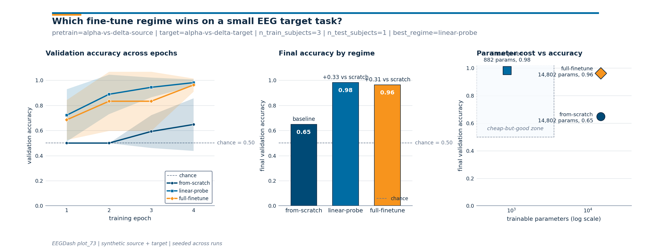
Result

The 3-panel figure folds the comparison three ways: per-epoch curves, final-accuracy bars on the same y-axis, and parameter cost vs accuracy in log-x. Drawing helpers live in a sibling _finetune_figure module so the plumbing stays out of the rendered tutorial.

from _finetune_figure import draw_finetune_figure

fig = draw_finetune_figure(
    epochs=EPOCH_AXIS,
    scratch_curve=curves["from-scratch"],
    probe_curve=curves["linear-probe"],
    finetune_curve=curves["full-finetune"],
    final_accuracies=final_accuracies,
    trainable_params=trainable_params,
    chance_level=chance,
    pretrain_task=PRETRAIN_TASK,
    target_task=TARGET_TASK,
    n_train_subjects=n_train_subjects,
    n_test_subjects=n_test_subjects,
)
plt.show()

A common mistake, and how to recover

Run. Reloading the encoder into a model whose n_chans differs raises a size-mismatch RuntimeError on the first conv. We trigger it with try/except so the failure mode is visible (Nederbragt et al. 2020, doi:10.1371/journal.pcbi.1008090).

try:
    # pretrained on 8 chans; rebuild with 10 to trip the size check.
    wrong = ShallowFBCSPNet(N_CHANS + 2, 2, n_times=N_TIMES, final_conv_length="auto")
    state = torch.load(ckpt_path, map_location="cpu", weights_only=True)
    wrong.load_state_dict(state, strict=True)
except RuntimeError as exc:
    print(f"Caught RuntimeError: {str(exc)[:90]}...")
    # Recovery: matching n_chans, strict=False, head re-init.
    fixed = build_model()
    missing, _ = fixed.load_state_dict(state, strict=False)
    head_only = all(k.startswith("final_layer") for k in missing)
    print(f"Recovery: matching n_chans + strict=False; head re-init={head_only}.")

Caught RuntimeError: Error(s) in loading state_dict for ShallowFBCSPNet:
        Missing key(s) in state_dict: "final_...
Recovery: matching n_chans + strict=False; head re-init=True.

Modify

Your turn. Add a fourth last-block regime: unfreeze the classifier conv and the final batch norm, pin the rest. The starter below switches requires_grad on for any name containing "conv_classifier" or "bnorm"; re-run the 3-seed loop and add a row to results_table.

last_block = build_model()
last_block.load_state_dict(
    torch.load(ckpt_path, map_location="cpu", weights_only=True), strict=False
)
for name, p in last_block.named_parameters():
    unfreeze = any(t in name for t in ("conv_classifier", "bnorm")) or (
        name.startswith("final_layer")
    )
    p.requires_grad = unfreeze
n_trainable = sum(p.numel() for p in last_block.parameters() if p.requires_grad)
print(
    f"last-block starter: trainable={n_trainable} "
    f"(linear-probe={trainable_params['linear-probe']}, "
    f"full-finetune={trainable_params['full-finetune']})"
)

last-block starter: trainable=962 (linear-probe=882, full-finetune=14802)

Mini-project

Replace the synthetic source/target with a real EEGDash query (one task for source, a different task for target on the same subject pool, mirrored from Pretrain on resting-state, fine-tune on contrast-change detection). Keep n_chans, n_times, and the optimiser fixed; replot the same 3-panel figure and compare gap-above-chance.

One JSON line carries the headline numbers a reviewer needs: which regime won, by how much over chance, by how much over from-scratch, and the trainable parameter cost.

best_name = max(final_accuracies, key=final_accuracies.get)
best_acc = final_accuracies[best_name]
print(
    json.dumps(
        {
            "pretrain_task": PRETRAIN_TASK,
            "target_task": TARGET_TASK,
            "n_train_subjects": n_train_subjects,
            "n_test_subjects": n_test_subjects,
            "best_regime": best_name,
            "best_accuracy": round(best_acc, 3),
            "chance_level": round(chance, 3),
            "gap_vs_chance": round(best_acc - chance, 3),
            "gap_vs_scratch": round(best_acc - final_accuracies["from-scratch"], 3),
            "trainable_params": trainable_params,
        }
    )
)

{"pretrain_task": "alpha-vs-delta-source", "target_task": "alpha-vs-delta-target", "n_train_subjects": 3, "n_test_subjects": 1, "best_regime": "linear-probe", "best_accuracy": 0.981, "chance_level": 0.5, "gap_vs_chance": 0.481, "gap_vs_scratch": 0.333, "trainable_params": {"from-scratch": 14802, "linear-probe": 882, "full-finetune": 14802}}

Wrap-up

We pretrained a Braindecode encoder, saved its weights, reloaded them into a fresh model with a replaced head, and compared three regimes on a leakage-safe cross-subject split. Every regime shared optimiser, batch size, schedule, and seeds; only the requires_grad mask differed. The split was subject-aware (leakage_report overlap=0), every RNG was seeded, and frozen + trainable == total held at every step. When the Braindecode foundation-model API stabilises, the only edits are to swap build_model + torch.load for from_pretrained(...) and call model.reset_head(n_outputs=K).

Try it yourself

• Vary pretraining length (1, 2, 5 epochs); does linear-probe climb faster?

• Swap ShallowFBCSPNet for EEGNetv4 and rerun the three regimes.

• Hold out two subjects and report mean +/- std across folds.

• Replace synth data with a windowed EEGDash query (/auto_examples/tutorials/10_core_workflow/plot_10_preprocess_and_window).

References

See References for the centralised bibliography of papers cited above. Add or amend an entry once in docs/source/refs.bib; every tutorial inherits the update.