


Note
Go to the end to download the full example code or to run this example in your browser via Binder.
Track 2: a public motor-imagery warm-up for session transfer#
Load BNCI2014-004 subject 1, sessions 0train and 1train, run 0 (nm000135). The two recordings total about 11 MB. This CPU baseline predicts observed left-hand and right-hand cues with log channel power. Session 0train fits the model; session 1train is held out without calibration. These are already processed real recordings. This compact motor-imagery example has two classes and its own session split, not the official three-command Graz / BrainHero protocol.
Source: https://nemar.org/dataset/nm000135
Before you start#
Use an installed EEGDash environment with Braindecode, MNE, NumPy,
scikit-learn and Matplotlib. This two-recording CPU example needs about 11 MB
of cached signal data. EEGDASH_CACHE_DIR chooses the persistent download
location; a network connection is needed when either session is absent.
The deployment question is prediction in another recorded session of the same person, without calibration on that session. The two labels are actual left- and right-hand imagery cues. This small BNCI corpus is an accessible example of session transfer; its two classes do not stand in for three mental commands.
What the official track asks, and what this example measures#
The 2026 track description specifies imagery, arithmetic and word-association commands across Graz and BrainHero contexts. The cohort has 20 people and six sessions each. Ten people supply all six labelled sessions; the other ten supply labelled sessions 1–3 for calibration and hidden sessions 4–6 for scoring. Evaluation averages balanced accuracy over subject/session/context cells. Combining every test window into one score could overweight cells with more data.
The NeuralBench Track 2 guide currently uses a public four-class Stieger motor-imagery task with a cross-subject split. It is a separate starter baseline, not the official cross-session protocol. This page uses a smaller two-class BNCI recording pair to exercise session separation through EEGDash. Its single held-out participant/session has no Graz/BrainHero context cells. Keep its score labelled as a local warm-up; neither extra classes nor contexts can be reconstructed by renaming its existing labels.
import matplotlib.pyplot as plt
import numpy as np
from braindecode.preprocessing import create_windows_from_events
from sklearn.linear_model import LogisticRegression
from sklearn.metrics import balanced_accuracy_score, ConfusionMatrixDisplay
from sklearn.pipeline import make_pipeline
from sklearn.preprocessing import StandardScaler

from eegdash.paths import get_default_cache_dir

from eegdash import EEGDashDataset
from eegdash.features import signal_variance
Inspect both sessions before preprocessing#
The explicit subject, session, run and task query should return exactly two recordings. Keeping session identities intact is essential: relabelling two runs as sessions would not test session generalization. The annotation printout confirms the available class names before defining their numeric codes.
C3, Cz and C4 cover the motor region and are the source’s three EEG channels.
The release is already processed; the additional 8–30 Hz filter selects the
sensorimotor frequency range for this particular power baseline rather than
claiming to redo acquisition preprocessing. MNE’s Raw.resample
converts to 100 Hz and reduces the
number of samples while retaining that passband. These fixed operations do not
learn their parameters from the held-out session, but the offline filtering
here should not be mistaken for causal streaming preprocessing.
# Native MNE resampling preserves annotations in seconds. No format conversion
# or manual event restoration is needed for this small three-channel recipe.

dataset = EEGDashDataset(
    dataset="nm000135",
    subject="1",
    session=["0train", "1train"],
    run="0",
    task="imagery",
    cache_dir=get_default_cache_dir(),
)
print(dataset.description.to_string(index=False))
for recording in dataset.datasets:
    raw = recording.raw.pick("eeg")
    # Limit RAM to three motor channels before filtering and resampling.
    raw.pick(["C3", "Cz", "C4"]).load_data().filter(8, 30)
    raw.reorder_channels(["C3", "Cz", "C4"]).resample(100)
subject session run    task  age sex hand   group species bci_experience gender
      1  0train   0 imagery 21.0   F    R healthy   human          naive   None
      1  1train   0 imagery 21.0   F    R healthy   human          naive   None
Reading 0 ... 604999  =      0.000 ...  2419.996 secs...
Filtering raw data in 1 contiguous segment
Setting up band-pass filter from 8 - 30 Hz

FIR filter parameters
---------------------
Designing a one-pass, zero-phase, non-causal bandpass filter:
- Windowed time-domain design (firwin) method
- Hamming window with 0.0194 passband ripple and 53 dB stopband attenuation
- Lower passband edge: 8.00
- Lower transition bandwidth: 2.00 Hz (-6 dB cutoff frequency: 7.00 Hz)
- Upper passband edge: 30.00 Hz
- Upper transition bandwidth: 7.50 Hz (-6 dB cutoff frequency: 33.75 Hz)
- Filter length: 413 samples (1.652 s)

Reading 0 ... 552499  =      0.000 ...  2209.996 secs...
Filtering raw data in 1 contiguous segment
Setting up band-pass filter from 8 - 30 Hz

FIR filter parameters
---------------------
Designing a one-pass, zero-phase, non-causal bandpass filter:
- Windowed time-domain design (firwin) method
- Hamming window with 0.0194 passband ripple and 53 dB stopband attenuation
- Lower passband edge: 8.00
- Lower transition bandwidth: 2.00 Hz (-6 dB cutoff frequency: 7.00 Hz)
- Upper passband edge: 30.00 Hz
- Upper transition bandwidth: 7.50 Hz (-6 dB cutoff frequency: 33.75 Hz)
- Filter length: 413 samples (1.652 s)
Window the actual imagery intervals#
left_hand and right_hand map explicitly to zero and one. After
resampling, 300 samples correspond to three seconds. Equal stride and window
size give non-overlapping complete windows within the labelled intervals;
on_last_window="drop" discards an incomplete remainder rather than padding
it. Zero start/stop offsets preserve the source event boundaries.
The window metadata carries session and target through preprocessing. Before
feature reduction, X has layout (windows, 3, 300) in volts. Natural-log
variance over time reduces it to one channel-power feature per channel. The
small numerical floor makes zero power finite, but does not perform artifact
rejection or rescue a noninformative electrode.
classes = {"left_hand": 0, "right_hand": 1}
windows = create_windows_from_events(
    dataset,
    mapping=classes,
    trial_start_offset_samples=0,
    trial_stop_offset_samples=0,
    window_size_samples=300,
    window_stride_samples=300,
    on_last_window="drop",
    preload=True,
)
metadata = windows.get_metadata()
X = np.stack([windows[i][0] for i in range(len(windows))])
y = metadata.target.to_numpy(dtype=int)
X = np.log(np.maximum(signal_variance(X), 1e-30))
Hold out a genuine session without recalibration#
Only 0train fits the model; 1train is the held-out session. Those
strings are source identifiers, not instructions to include both in training.
The two sessions share a participant intentionally and contain the same
observed two-class task.
Feature standardization belongs inside the pipeline so the test-session mean
and variance remain unseen during fitting. Logistic regression uses its default
regularization; max_iter=1000 gives the optimizer room to converge and is
not a score-tuning parameter. This page has no validation set and therefore
makes no data-driven hyperparameter selection.
train = metadata.session.eq("0train").to_numpy()
test = metadata.session.eq("1train").to_numpy()
print("Features:", X.shape, "classes:", np.unique(y, return_counts=True))
Features: (240, 3) classes: (array([0, 1]), array([120, 120]))
model = make_pipeline(StandardScaler(), LogisticRegression(max_iter=1000))
predicted = model.fit(X[train], y[train]).predict(X[test])
print(
    "Held-out session balanced accuracy:", balanced_accuracy_score(y[test], predicted)
)
print("Constant-class balanced-accuracy reference: 0.5")
ConfusionMatrixDisplay.from_predictions(
    y[test], predicted, display_labels=list(classes)
)
plt.xticks(rotation=25)
plt.tight_layout()
plt.show()
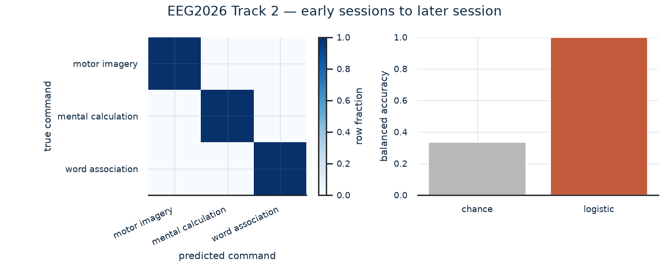
Held-out session balanced accuracy: 0.5333333333333333
Constant-class balanced-accuracy reference: 0.5
Interpret session transfer and extend it#
Balanced accuracy is the mean of left-hand and right-hand recall, with 0.5 as the uniform two-class reference. The confusion matrix displays actual counts: inspect whether errors concentrate in one class instead of relying on a single score. A near-chance result can reflect a weak feature representation or real session differences; it should not trigger a favourable-score assertion.
One person’s two sessions do not establish population performance. To tune the band range, regularization or an EEGNet model, add a separate validation session and preserve the present test session. Then repeat the design across additional people where the catalogue actually supplies the required sessions. Compare pipelines using identical held-out windows and retain original trial IDs if extracting several windows from each trial.
To move to the official task, use the released command labels and session assignments from the competition source, retain participant/context metadata, and compute the per-cell metric before averaging. Keep later sessions out of calibration and hyperparameter selection. Changing the classifier output size alone would not make this two-class dataset an official evaluation.
Related worked example: Braindecode cross-session motor imagery.
